H1

Setup

Document Rendering

(Detailed document rendering options not shown)

R Packages

library(glue)        # formatting strings
library(lubridate)   # parsing datetime information
library(kableExtra)  # table formatting      
library(httr)        # or curl, httr, or rvest?
library(xml2)
library(tidyverse)   # powerful data processing
theme_set(theme_bw())# white background

1
2
3
4
5
6
7

setwd(here::here("/home/knut/code/git/_my/work/dis-docs/"))
setwd(here::here("guide/internal"))

1
2

Get metadata formats

url_mdfmt="https://doidb.wdc-terra.org/igsnoaip/oai?verb=ListMetadataFormats"

md_fmt <- xml2::read_xml(url_mdfmt,  as_html = FALSE,  options = "NOBLANKS") %>% 
    xml_ns_strip() %>% 
    xml2::xml_find_all(xpath = ".//metadataPrefix", ns = xml_ns(.)) %>% 
    xml2::xml_text(x = .)

1
2
3
4
5
6

Metadata_formats are: oai_dc, igsn.

Get Sets/Metadata Catalogs

url_doi="https://doidb.wdc-terra.org/igsnoaip/oai?"
url_sets="verb=ListSets"

url_catalogs <- sprintf("%s%s", url_doi, url_sets)
catalogs <- xml2::read_xml(url_catalogs) %>% 
  xml_ns_strip() 

setnames <- catalogs %>%   
  xml2::xml_find_all(xpath = ".//setName", ns = xml_ns(.)) %>% 
  xml_text() 

setspecs <- catalogs %>%   
  xml2::xml_find_all(xpath = ".//setSpec", ns = xml_ns(.)) %>% 
  xml_text() 
  
catalogs_df <- tibble(name = setnames, spec = setspecs) %>% 
  filter(str_detect(.$name, "(?i)Reference quality citations only", negate = TRUE) )

1
2
3
4
5
6
7
8
9
10
11
12
13
14
15
16
17

Calculate a data frames of year-intervals

n <- 2009
n_years <-  lubridate::year(Sys.Date())
years <- tibble(year = seq(n, n_years))
dates_intervals <- years %>% 
  mutate(doy_first = sprintf("%s-01-01", year),
         doy_last =  sprintf("%s-12-31", year))

1
2
3
4
5
6

n_rows <- nrow(dates_intervals)
n_last <- n_rows - 2
dates_intervals %>% 
  rownames_to_column(var = "#") %>% 
  slice(c(seq(1,3), seq(n_last, n_rows))) %>% 
  knitr::kable(row.names = TRUE) %>%
  kableExtra::kable_styling(., bootstrap_options = "striped")

1
2
3
4
5
6
7

	#	year	doy_first	doy_last
1	1	2009	2009-01-01	2009-12-31
2	2	2010	2010-01-01	2010-12-31
3	3	2011	2011-01-01	2011-12-31
4	12	2020	2020-01-01	2020-12-31
5	13	2021	2021-01-01	2021-12-31
6	14	2022	2022-01-01	2022-12-31

Goal: Run HTTP GET request for each catalog - year combination.

Step 1/3: Prepare a dataframe of http-calls to verb/method verb=ListSets`

url_records = "verb=ListRecords"

url_records_tpl <- glue::glue("{url_doi}{url_records}&metadataPrefix=oai_dc")

http_requests <- catalogs_df %>% 
  crossing(dates_intervals) %>% 
  mutate(req = glue("{url_records_tpl}&from={doy_first}&until={doy_last}&set={spec}"))

1
2
3
4
5
6
7

Step 2/3: Now compose getter function for fetchin XML Data via HTTP.

#  purrr:partial
status_extract <- compose(httr::status_code, httr::GET)

find_all <- partial(xml2::xml_find_all, xpath = ".//resumptionToken/@completeListSize")


get_count <- compose(possibly(xml2::xml_text, otherwise = "0"), 
                       possibly(find_all,  otherwise = "0"),
                       possibly(xml_ns_strip, otherwise = "0"),
                       possibly(xml2::read_xml, otherwise = "0"))

1
2
3
4
5
6
7
8
9
10

Step 3/3: Use the xml getter function to extend the dataframe of URLs with the count of DOIS assigned per year.

This will perform 350 HTTP requests (for all 14 years * 25 catalogs),

outfile_rds <- "../../assets/other/data/igsns_per_year.RDS"
if (file.exists(outfile_rds)) {
  #igsns_per_year <- readRDS(outfile_rds)
  igsns_per_year <- readRDS(outfile_rds)
} else {
  igsns_per_year <- http_requests %>% 
    mutate(cnt = map(req, get_count)) 
  saveRDS(igsns_per_year, file = outfile_rds)
}

1
2
3
4
5
6
7
8
9

n_rows <- nrow(igsns_per_year)
n_last <- n_rows - 4

igsns_per_year %>% 
  arrange(year, name) %>% 
  rownames_to_column(var = "#") %>% 
  slice(c(seq(1,3), seq(n_last, n_rows))) %>% 
  knitr::kable(row.names = TRUE) %>%
  kableExtra::kable_styling(., bootstrap_options = "striped")

1
2
3
4
5
6
7
8
9

	#	name	spec	year	doy_first	doy_last	req	cnt
1	1	AuScope	ANDS.AUSCOPE	2009	2009-01-01	2009-12-31	https://doidb.wdc-terra.org/igsnoaip/oai?verb=ListRecords&metadataPrefix=oai_dc&from=2009-01-01&until=2009-12-31&set=ANDS.AUSCOPE
2	2	AuScope Geochemistry Network	LITHODAT.AG	2009	2009-01-01	2009-12-31	https://doidb.wdc-terra.org/igsnoaip/oai?verb=ListRecords&metadataPrefix=oai_dc&from=2009-01-01&until=2009-12-31&set=LITHODAT.AG
3	3	Australian National Data Service	ANDS	2009	2009-01-01	2009-12-31	https://doidb.wdc-terra.org/igsnoaip/oai?verb=ListRecords&metadataPrefix=oai_dc&from=2009-01-01&until=2009-12-31&set=ANDS
4	346	MARUM Center for Marine Environmental Sciences	MARUM.HB	2022	2022-01-01	2022-12-31	https://doidb.wdc-terra.org/igsnoaip/oai?verb=ListRecords&metadataPrefix=oai_dc&from=2022-01-01&until=2022-12-31&set=MARUM.HB	1
5	347	MARUM Center for Marine Environmental Studies at University of Bremen	MARUM	2022	2022-01-01	2022-12-31	https://doidb.wdc-terra.org/igsnoaip/oai?verb=ListRecords&metadataPrefix=oai_dc&from=2022-01-01&until=2022-12-31&set=MARUM	1
6	348	System for Earth Sample Registration	IEDA.SESAR	2022	2022-01-01	2022-12-31	https://doidb.wdc-terra.org/igsnoaip/oai?verb=ListRecords&metadataPrefix=oai_dc&from=2022-01-01&until=2022-12-31&set=IEDA.SESAR	59771
7	349	Universität Kiel	UKI	2022	2022-01-01	2022-12-31	https://doidb.wdc-terra.org/igsnoaip/oai?verb=ListRecords&metadataPrefix=oai_dc&from=2022-01-01&until=2022-12-31&set=UKI
8	350	Universität Kiel - Rechenzentrum	UKI.RZ	2022	2022-01-01	2022-12-31	https://doidb.wdc-terra.org/igsnoaip/oai?verb=ListRecords&metadataPrefix=oai_dc&from=2022-01-01&until=2022-12-31&set=UKI.RZ

Done with getting data.

Prepare data for plotting

Remove those catalogs that contanin a "." in their setSpec attribute.
They are subcatalogs, and often there is only 1 subcatalog for each registrant.

Add a few columns to make calculations and plotting easier.

igsns_per_year_clean <- igsns_per_year %>% 
  arrange(spec, doy_last) %>% 
  mutate(cnt =  as.integer(cnt)) %>% 
  filter(str_detect(spec, "\\.", negate = TRUE)) %>% # remove "subcatalogs". 
  mutate(
         year2 = as.Date(glue("{year -1}-12-31")),
         spec2 = spec,
         spec2 = fct_reorder(spec2, -cnt, sum, na.rm = TRUE),
         catalog = as.factor(case_when(
    spec2 == "GEOAUS" ~ "GEO AUS",
    spec2 == "IEDA" ~ "SESAR",
    #spec2 == "GFZ" ~ "GFZ",
    TRUE ~ "(other)"
         )))
  
igsns_per_year_max <- igsns_per_year_clean %>% 
  arrange(spec, doy_last) %>% 
  filter(!is.na(cnt)) %>% 
  select(spec, year, cnt) %>% 
  group_by(spec) %>% 
  summarize(maxcnt = max(cnt, na.rm = TRUE)) %>% 
  ungroup() %>% 
  mutate(max_yearly = as.factor(case_when(
    maxcnt >= 10000 ~ ">= 10000",
    maxcnt >= 1000 ~ " >=  1000",
    TRUE ~ "<=  1000"
         )),
        max_yearly = fct_relevel(max_yearly, ">= 10000", " >=  1000", "<=  1000")) %>% 
  select(-maxcnt) 
  

igsns_per_year_clean <- igsns_per_year_clean %>% 
  inner_join(igsns_per_year_max, by = "spec")

igsns_per_year_sm <- igsns_per_year_clean %>% 
  filter(catalog == "(other)" )

1
2
3
4
5
6
7
8
9
10
11
12
13
14
15
16
17
18
19
20
21
22
23
24
25
26
27
28
29
30
31
32
33
34
35
36

Plots

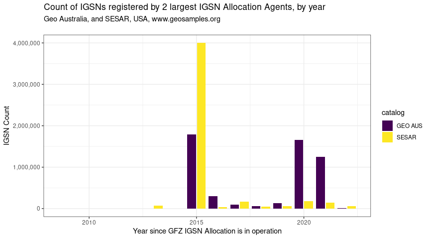
p01_total <- igsns_per_year_clean %>% 
  filter(catalog != "(other)" ) %>% 
  filter(year >= 2009) %>% 
  ggplot(aes(year2, cnt, fill = catalog)) +
  geom_bar(stat = "identity", position = "dodge2") +
  #theme(legend.position = "none") +
  #annotate("text", x = as.Date("2017-12-31"), y = 3000, label = "turquoise = IGSNs of GEOFON records, 2013-2015\nred = IGSNs in all other catalogs") + 
  scale_x_date() + 
  scale_y_continuous(labels = scales::label_comma()) + 
  scale_fill_viridis_d() +
  labs(x = "Year since GFZ IGSN Allocation is in operation",
       y = "IGSN Count",
       title = "Count of IGSNs registered by 2 largest IGSN Allocation Agents, by year",
       subtitle = "Geo Australia, and SESAR, USA, www.geosamples.org\n")
p01_total

1
2
3
4
5
6
7
8
9
10
11
12
13
14
15

igsn_svg <- "img/igsn_svg_p01_total.svg"
ggsave(file = igsn_svg, plot = p01_total, width = 10, height = 8)

1
2

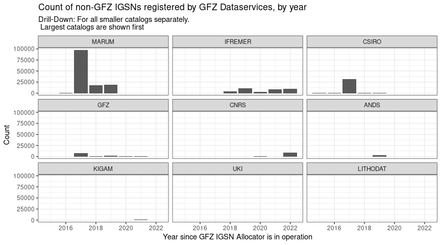
Smaller IGSN catalogs, Sorted by total number of records

p02_separate <- igsns_per_year_sm %>% 
  ggplot(aes(year2, cnt)) +
  geom_col() +
  scale_x_date() + 
  labs(x = "Year since GFZ IGSN Allocator is in operation",
       y = "Count",
       title = "Count of non-GFZ IGSNs registered by GFZ Dataservices, by year",
       subtitle = "Drill-Down: For all smaller catalogs separately.\n Largest catalogs are shown first") +
  facet_wrap(~spec2)
p02_separate

1
2
3
4
5
6
7
8
9
10

igsn_svg <- "img/igsn_svg_p02_separately_absolute.svg"
ggsave(file = igsn_svg, plot = p02_separate, width = 10, height = 8)

1
2

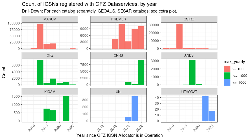
Smaller IGSN Catalogs, with individual Y-Axis scales

Same plot as before, zoomed in, with individual Y-Axis scales, and subplots sorted by total number of records:

p03_classifc <- igsns_per_year_sm %>% 
  ggplot(aes(year2, cnt, color = max_yearly, fill = max_yearly)) +
  geom_col() +
  theme(axis.text.x = element_text(angle=45, hjust = 1)) +
  labs(x = "Year since GFZ IGSN Allocator is in Operation",
       y = "Count",
       title = "Count of IGSNs registered with GFZ Dataservices, by year",
       subtitle = "Drill-Down: For each catalog separately. GEOAUS, SESAR catalogs: see extra plot.") +
  facet_wrap(~spec2, scales = "free_y")
p03_classifc

1
2
3
4
5
6
7
8
9
10

igsn_svg <- "img/igsn_svg_p03_with_classific.svg"
ggsave(file = igsn_svg, plot = p03_classifc, width = 10, height = 8)

1
2